


This is the first article I wanted to publish when I started writing about the technology behind The Witness. I had just spent a week or so implementing irradiance caching with rotation and translation gradients. Extending the equations of the gradient estimation to the hemicube sample distribution had proven to be tricky and had taken me a considerable amount of effort. So, I thought it would be cool to document my derivation, so that others would not have to do the same. However, for that article to make sense I first had to provide some background, hence the previous two articles:
Unfortunately, by the time I was done with these, the work I had done on the gradients was not so fresh anymore, which is why it has taken me so long to complete this article.
In my previous post I mentioned the need to find an algorithm that would allow us to extrapolate the irradiance to fill lightmap texels with invalid samples, to smooth the resulting lightmaps to reduce noise, and to sample the irradiance at a lower frequency to improve performance. As some avid readers suggested Irradiance Caching solves all these problems. However, at the time I didn't know that, and my initial attempts at a solution were misguided.
Texture Space Approaches
I had some experience writing baker tools to capture normal and displacement maps from high resolution meshes. In that setting it is common to use various image filters to fill holes caused by sampling artifacts and extend sampled attributes beyond the boundaries of the mesh parameterization. Hugo Elias' popular article also proposes a texture space hierarchical sampling method, and that persuaded me that working in texture space would be a good idea.
However, in practice texture space methods had many problems. Extrapolation filters only provide accurate estimates close to chart boundaries, and even then, they only use information from one side of the boundary, which usually results in seams. Also, the effectiveness of irregular sampling and interpolation approaches in texture space is greatly reduced by texture discontinuities and did not reduce the number of samples as much as desired.
After trying various approaches, it became clear that the solution was to work in object space instead. I was about to implement my own solution, when I learned that this is what irradiance caching was about.
Irradiance Caching
This technique has such a terrible name that I would have never learned about it if it wasn't due to a friend's suggestion. I think that a much more appropriate name would be adaptive irradiance sampling or irradiance interpolation. In fact, in the paper that introduced the technique for the first time Greg Ward referred to it as lazy irradiance evaluation, which seems to me a much more appropriate name.
There's plenty of literature on the subject and I don't want to repeat what you can learn elsewhere. So, in this article I'm only going to provide a brief overview, focus on the unique aspects of our implementation, and point you to other sources for further reference.
The basic idea behind irradiance caching is to sample the irradiance adaptively based on a metric that predicts changes in the irradiance due to proximity to occluders and reflectors. This metric is based on the split sphere model, which basically models the worst possible illumination conditions in order to predict the necessary distance between irradiance samples based on their distance to the surrounding geometry.
Interpolation between these samples is then performed using radial basis functions, the radius associated to each sample is also based on this distance. Whenever the contribution of the nearby samples falls below a certain threshold a new irradiance record needs to be generated, in our case this is done by rendering an hemicube at that location. In order to perform interpolation efficiently the irradiance records are inserted in an octree, which allows us to efficiently query the nearby records at any given point.
For more details, the Siggraph '08 course on the topic is probably the most comprehensive reference. There's also a book based on the materials of the course; it's slightly augmented, but in my opinion it does not add much value to the freely available material.
The Physically Based Rendering book by Matt Pharr & Greg Humphreys is an excellent resource and the accompanying source code contains a good, albeit basic implementation.
Finally, Rory Driscoll provides a good introduction from a programmer's point of view: part 1, part 2.
Our implementation is fairly standard, there are however a two main differences: First, we are sampling the irradiance using hemicubes instead of a stratified Montecarlo distribution. As a result, the way the we compute the irradiance gradients for interpolation is somewhat different. Second, we use a record placement strategy more suited to our setting. In part 1 I'll focus on the estimation of the irradiance gradients, while in part 2 I'll write about our record placement strategies.
Irradiance Gradients
When interpolating our discrete irradiance samples using radial basis functions the resulting images usually have spotty or smudgy appearance. This can be mitigated by increasing the number of samples and increasing the interpolation threshold, which effectively makes them overlap and smoothes out the result. However, this also increases the number of samples significantly, which defeats the purpose of using irradiance caching.
One of the most effective approaches to improve the interpolation is estimating the irradiance gradients at the sampling points, which basically tell how the irradiance changes when the position and orientation of the surface changes. We cannot evaluate the irradiance gradients exactly, but we can find reasonable approximations with the information that we already have from rendering an hemicube.
In my previous article I explained that the irradiance integral was just a weighted sum over the radiance samples, where the contribution of each sample is the product of the radiance through each of the hemicube texels 


")

 \simeq \sum_{i=0}^N A_i L_i \cos\theta_i")
The irradiance gradients consider how each these terms change under infinitesimal rotations and translations and can be obtained by differentiating
 \simeq \sum_{i=0}^N \nabla A_i L_i \cos\theta_i")
The radiance term is considered to be constant, so the equation reduces to:
 \simeq \sum_{i=0}^N L_i \nabla A_i \cos\theta_i")
In reality, the radiance is not really constant, but the goal is to estimate the gradients without using any information in addition to what we have already obtained by rendering the scene on a hemicube. So that we can improve the quality of the interpolation by only doing some additional computations while integrating the hemicube.
Rotation Gradient
The rotation gradient expresses how the irradiance changes as the hemicube is rotated in any direction:
 \simeq \sum_{i=0}^N L_i \nabla_r A_i \cos\theta_i")
The most important observation is that as the hemicube rotates, the solid angle of the texels with respect to the origin remains constant. So, the only factor that influences the gradient is the cosine term:

With this in mind, the rotation gradient is simply the rotation axis scaled by the rate of change, that is, the angle gradient:

And the rotation axis is given by the cross product of the z axis and the texel direction 
 \right|")
Therefore:

This can be simplified further by noting that 

")
Finally, the rotation gradient for the hemisphere is the sum of the gradients corresponding to each texel.
 \simeq \sum_{i=0}^N L_i A_i (\mathbf{d}_{yi}, -\mathbf{d}_{xi}, 0)")
The resulting code is trivial:
foreach texel, color in hemicube { Vector2 v = texel.solid_angle * Vector2(texel.dir.y, -texel.dir.x); rotation_gradient[0] += v * color.x; rotation_gradient[1] += v * color.y; rotation_gradient[2] += v * color.z; } |
Translation Gradients
The derivation of the translation gradients is a bit more complicated than the rotation gradients because the solid angle term is not invariant under translations anymore.
My first approach was to simplify the expression of the solid angle term by using an approximation that is easier to differentiate. Instead of using the exact texel solid angle like I had been doing so far, I approximated it by the differential solid angle scaled by the constant area of the texel, which is a reasonable approximation if the texels are sufficiently small.
In general, the differential solid angle in a given direction 

For the particular case of the texels of the top face of the hemicube, n is equal to the z axis. So, the differential solid angle is:

We also know that:

which simplifies the expression further:
^3 da")
Using this result and factoring the area of the texels out of the sum we obtain the following expression for the gradient:
 \simeq 4 \sum_{i=0}^N L_i \nabla_t (\cos\theta_i)^4")
The remaining faces have similar expressions, slightly more complex, but still easy to differentiate along the x and y directions. We could continue along this path and we would obtain closed formulas that can be used to estimate the translation gradients. However, this simple approach did not produce satisfactory results. The problem is that these gradients assume that the only thing that changes under translation is the projected solid angle of the texels, but that ignores the parallax effect and the occlusion between neighboring texels. That is, samples that correspond to objects that are close to the origin of the hemicube should move faster than those that that are farther, and as they move they may occlude nearby samples.
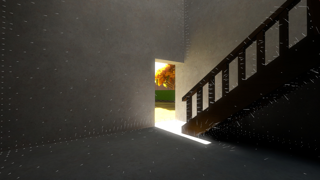
As you can see in the following lightmap, the use of these gradients resulted in smoother results in areas that are away from occluders, but produced incorrect results whenever the occluders are nearby.
Left: Reference. Middle: Irradiance caching without gradients. Right: Irradiance caching with flawed gradients
The hexagonal shape corresponds to the ceiling of a room that has walls along its sides and a window through which the light enters. The image on the left is a reference lightmap with one hemicube sample per pixel. The image on the middle is the same lightmap computed using irradiance caching taking only 2% of the samples. Note that the number of samples is artificially low to emphasize the artifacts. On the right side the same lightmap is computed using the proposed gradients. If you look closely you can notice that on the interior the lightmap looks smoother, but close to the walls the artifacts remain.
This is exactly the same flaw of the gradients that Krivanek et al proposed in Radiance Caching for Efficient Global Illumination Computation, but was later corrected in the followup paper Improved Radiance Gradient Computation by approaching the problem the same way Greg Ward did in the original original Irradiance Gradients paper.
I then tried follow the same approach. The basic idea is to consider the cosine term invariant under translation so that only the area term needs to be differentiated, and to express the gradient of the cell area in terms of the marginal area changes between adjacent cells. The most important observation is that the motion of the boundary between cells is always determined by the closest sample, so this approach takes occlusion into account.
Unfortunately we cannot directly use Greg Ward's gradients, because they are closely tied to the stratified Montecarlo distribution and we are using a hemicube sampling distribution. However, we can still apply the same methodology to arrive to a formulation of the gradients that we can use in our setting.
In our case, the cells are the hemicube texels projected onto the hemisphere and the cell area is the texel solid angle. To determine the translation gradients of the texel's solid angle is equivalent to computing the sum of the marginal gradients corresponding to each of the texel walls.
These marginal gradients are the wall normals projected onto the translation plane, scaled by the length of the wall, and multiplied by the rate of motion of the wall in that direction.
Since the hemicube uses a gnomonic projection, where lines in the plane map to great circles in the sphere, the texel boundaries of the hemicubes map to great arcs in the hemisphere. So, the length of these arcs is very easy to compute. Given the direction of the two texel corners 
 = \arccos{\mathbf{d}_0 \cdot \mathbf{d}_1}")
The remaining problem is to compute the rate of motion of the wall, which as Greg Ward noted has to be proportional to the minimum distance of the two samples.
The key observation is that we can classify all the hemicube edges in wo categories: Edges with constant longitude (

In each of these cases we can estimate the rate of change of edges with respect to the normal direction by considering the analogous problem in the canonical hemispherical parametrization:


For longitudinal edges we can consider how

and for latitudinal edges we can consider how

As we noted before, the rate of the motion is dominated by the nearest edge, so 
A detailed derivation for these formulas can be found in Wojciech Jarosz's dissertation, which is now publicly available online. His detailed explanation is very didactic and I highly recommend reading it to get a better understanding of how these formulas are obtained.
Note that these are just the same formulas used by Greg Ward and others. In practice, the only thing that changes is the layout of the cells and the length of the walls between them.
As can be seen in the following picture, the new gradients produce much better results. Note that the appearance on the interior of the lightmap is practically the same, but closer to the walls the results are now much smoother. Keep in mind that artifacts are still present, because the number of samples is artificially low.
Left: No gradients. Middle: Flawed translation gradients. Right: Improved translation gradients.
In order to estimate the translation gradients efficiently we precompute the direction and magnitude of the marginal gradients corresponding to each texel edge without taking the distance to the edge into account:
// Compute the length of the edge walls multiplied by the rate of motion // with respect to motion in the normal direction foreach edge in hemicube { float wall_length = acos(dot(d0, d1)); Vector2 projected_wall_normal = normalize(cross(d0, d1).xy); float motion_rate = (constant_altitude(d0,d1) ? -cos_theta(d0,d1) : // d(theta)/dx = -cos(theta) / depth -1 / sin_theta(d0,d1); // d(phi)/dy = -1 / (sin(theta) * depth) edge.translation_gradient = projected_wall_normal * wall_length * motion_rate; } |
Then, during integration we split the computations in two steps. First, we accumulate the marginal gradients of each of the edges scaled by the minimum edge distance:
foreach edge in hemicube { float depth0 = depth(edge.x0, edge.y0); float depth1 = depth(edge.x1, edge.y1); float min_depth = min(depth0, depth1); texel[edge.x0, edge.y0].translation_gradient -= edge.gradient / min_depth; texel[edge.x1, edge.y1].translation_gradient += edge.gradient / min_depth; } |
Once we have the per texel gradient, we compute the final irradiance gradient as the sum of the texel gradients weighted by the texel colors:
foreach texel, color in hemicube { Vector2 translation_gradient = texel.translation_gradient * texel.clamped_cosine; translation_gradient_sum[0] += translation_gradient * color.x; translation_gradient_sum[1] += translation_gradient * color.y; translation_gradient_sum[2] += translation_gradient * color.z; } |
Conclusions
Irradiance Caching provides a very significant speedup to our lightmap baker. On typical meshes we only need to render about 10 to 20% of the samples to approximate the irradiance at very high quality, and for lower quality results or fast previews we can get away with as few as 3% of the samples.
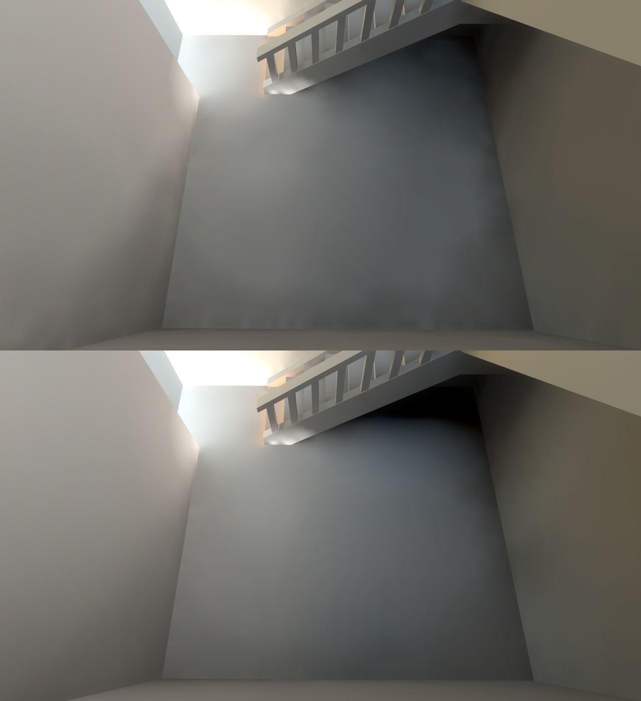
The use of irradiance gradients for interpolation allows reducing the number of samples significantly, or for the same number of samples produces much higher quality results. The following picture compares the results without irradiance gradients and with them, in both cases the number of samples and their location is the same, note how the picture at the bottom has much smoother lightmaps.
I think that without irradiance caching the hemicube rendering approach to global illumination would have not been practical. That said, implementing irradiance caching robustly is tricky and a lot of tuning and tweaking is required in order to obtain good results.
Note: This article is also published on #AltDevBlogADay.
This is a really great article Ignacio! Thanks very much. I look forward to the second one.
You already be aware of this, and it doesn’t really affect your lightmap baker, but I believe one problem with irradiance caching is temporal stability. If you render multiple frames with moving lights you tend to get popping as different adaptation decisions are made. I think there are alternatives for this, but I forget the references. Anyway, just thought I’d mention it.
ta,
Sam
Temporal stability is not a great concern for us, because our lightmaps are static. In some areas we have multiple lightmaps for different lighting configurations and simply blend between then. In that case Irradiance Caching could introduce some stability artifacts, but that is not very noticeable as long as the quality of the lightmaps is high enough.
Note that I have no idea what I’m talking about here and maybe I’m missing something important. For example, it took me multiple re-reads to decipher what you were saying enough to actually even see where the depth values of the hemicube samples were being used in computing the gradients.
Anyway, ignoring rotation, I assume what you’re computing with these gradients is a linear extrapolation, something like: E(X+dx) = E(X) + u*dEdu + v*dEdv. Whatever this formula turns out to be, I would think the task isn’t actually to compute infinitesimal gradients at X, but to compute the optimal numbers that supposedly are “dEdu” and “dEdv” that allow you to extrapolate as far as possible (e.g. in a least squares sense). One could hypothesize some sort of higher-order extrapolation as well, and it might be more tractable under this model where you’re not looking at gradients, but looking at it as generating approximating polynomials or some such. However I don’t know what the math would look like for trying to model things this way. It just seems a weird thing to me to start off with the gradients. (I guess this is a basic well-known thing; the gradient is a particular truncated Taylor series to the actual function. But truncating a Taylor series doesn’t actually give the best approximation for that order.)
I’m not sure how gradient rotation can work when you have a hemisphere(cube) of samples instead of a sphere of samples. Is this only used for small rotations (e.g. on a curved surface) and not at large rotations (e.g. a 30-degree joint)? Is it only used at internal angles (where visibility means less than a hemisphere is actually visible anyway, so nothing is missing) and not at external angles (where there can be missed samples “around the corner”)?
Yeah, Jon also suggested I added a section explaining how the gradients are used, I thought it was a good idea as it would clarify things a bit, but our implementation is completely standard in that regard, and time for my #AltDevBlogADay post was running out (in fact I was 1.5 hours late), so that got cut out.
I think you have a good point, but you have to keep in mind that this whole thing is a very crude approximation anyway. As you translate your sampling point new radiance sources that were previously occluded could come into view. The same thing happens with rotations, sources below the horizon may become visible under rotation. These effects are largely ignored, but despite of that the approximation provides better results than using no approximation at all, and it does so at a very small cost.
Keep in mind that the approximations are only OK with very small rotations and translations. One of the things that are also estimated when analyzing the hemicubes is how accurate are the approximation expected to be, and this is used to guide the record placement.
Sometimes the estimates fail miserably and that results in artifacts. This usually happens under translations, when a bright radiance source becomes suddenly visible. Existing methods don’t deal very well with this scenario and I think I came up with a innovative solution to the problem. Rotations are usually not an issue, because the radiance samples are cosine weighted, so the new samples that appear near the horizon have near-zero weight.
I personally think there’s still quite a bit of room for innovation on this area, but I pretty much limited myself to adapt the existing methods to our setting and work around the problems that we found. Once our implementation was working well enough I just moved on, since we have many other things to do that have a much bigger impact on the final game.
Ok, fair enough. In the sample shot at the top the sample points seem pretty far apart, but maybe that was captured with the same “exagerrated to show you the effect” settings.
I guess another question is to what degree the look with correctly tuned settings has any visible mottling which isn’t actually present if you don’t do caching. I’m not experienced enough with radiosity to know what things “should” look like. Is it tuned so there’s no visible effect? Or is it subtly visible but acceptable?
That shot is actually using our default settings and corresponds to the lightmap view at the end of the post, which I think does not have obvious artifacts. In that shot the minimum distance between samples is limited by the lightmap resolution. The samples that are farther apart, are so, because they are far enough from occluders, and because the irradiance is not expected to change abruptly. I basically tweaked our error thresholds to get the desired visual results at the minimum cost and that results in the sample distribution depicted in the screenshot.
With our high quality/production settings, artifacts are gone entirely, and at the medium/default settings they are rarely noticeable. Note, that our results are biased, we trade accuracy/correctness for smoothness/good appearance. In fact, some of the scenes that looked noisy without caching (due to the limited hemicube resolution), looked much better with caching enabled.
Nice article :)
fwiw– the siggraph course link is broken … looks like it’s moved to here: http://cgg.mff.cuni.cz/~jaroslav/papers/2008-irradiance_caching_class/index.htm
Thanks! I updated the link.
When developers get all technical… is good! but i don’t understand…
So this is for saving space? so that the game is not as heavy to download or so that it loads faster or to not include load screens?
Is this used often? do other games have it? is it popular or used in AAA games or no other game has this, is this revolutionary, will it help games get easier to develop in the future… ?
i don’t know if this is new for real time graphics, but if its not… you guys have ton of friends in the industry. why not just ask for help? i don’t know about the ethics of game development or if you can use what someone told you but maybe you just don’t believe that other games use it right? so you have to go through all this yourself…
That would be a cool post to see! “Ethics of Game Design and Asking for Help”
Cool new tech you’re working on there. But about the game. Is it related to Infocom’s The Witness. Inspired perhaps, or just a coincidental name? See the link for ‘my website’ (not actually mine) for further info.
“We’ve just started showing the game to the press; after Monday the 8th they may start talking about it. Who can say?”
Will links to articles be posted here… i can never find out about indie games coverage. N4G doesn’t like indie games and a lot of hub news site never post previews on indies, but if i found news of the game from other sites i will not only share them here but i will try to publish it at N4G and other hubs.
Also, will The Witness have a story that is heavy on Science and Science Fiction like Braid was?
I love the story of Braid and it thought me the importance of science in the world and the importance of getting serious about the objective world, but at the same time looking at things from many angles from a subjective perspective.
Like making an atomic bomb or going to space, i hope the story is about deep and meaningful things to the human race. i hope , like Braid can get me even more interested in science!
Also… who is the voice actor? is it the same guy that did the tutorial from Raspberry, he had a charming voice! is he your friend or something?
Justin – part of me feels that even if the game hasn’t any direct storytelling in it, there will be loads of implicit story and meaning in every piece of the puzzle. The Witness as a title reminds me of buddhism – buddha meaning in many ways “the witness.” The awakened one who observes. It is very much part of zen philosophy to be a silent observer, and that may be the player’s role in this game. I wouldn’t be surprised if it were up to us to infer meaning on our own… and if so, I think it will make the game so much more amazing. :)
Guys… you are like the most technical people i could think of showing this to. When I first saw this about a year ago i thought it was a scam to make people invest in false technology nut now those guys have come up with another demo.
http://www.youtube.com/watch?v=00gAbgBu8R4&feature=channel_video_title
Ignacio, Jonathan… is this for real? if so why isn’t anyone talking about it or investing or trying to replicate it? Ignacio worked for Nvidia, right? are those guys looking into anything similar?
a year ago they showed and earlier demo and they got some attention. mostly from people that said it was not true or just a joke or whatever, but why would they come back? I mean if nothing can run this why bother?
http://www.youtube.com/watch?v=Q-ATtrImCx4 (year old demo)
http://www.baytallaah.com/osholibrary/reader.php?endpos=22012&page=11&book=Kyozan%20-%20A%20True%20Man%20of%20Zen
Here is a link to a page in a book. I was listening to a reading the other day by its author, Osho, and thought of this game. I can only hope there is some relation. Even if not, I’m sure the curious player will still be able to create their own interpretation.
Pingback: Irradiance Caching – Continued | Ignacio Castaño
Ignacio this article is one of the best Irradiance caching resources on the internet, unfortunately in its current form with all the equations missing, it’s also one of the biggest computer graphics troll articles on the internet =)
Look at all of these amazing results to this really hard problem you are facing but all the equations are gone! Is there any way to revive the equations?
At the moment, it does seem that you can still see the equations on the internet archive version: https://web.archive.org/web/20130121205251/http://the-witness.net/news/2011/07/irradiance-caching-part-1/
Should be fixed now! We are using a plugin that converts LaTeX code into a .png and it was defaulting to white on white. Can you guys read it well now?
Looks good. :)