


During the last several weeks I've been polishing and optimizing the shadowing system and I think that at this point it won't undergo any more significant changes. In the process I've been reading a bit and looking up references and I'm appalled by how inaccessible is all the shadow mapping knowledge. For the most part it is scattered in obscure power point presentations, random some blog posts, SDK examples from Microsoft and hardware vendors (NVIDIA, AMD, Intel), and numerous ShaderX / GPU Gems / GPU Pro books.
I'm not going to try to address that here, but just as I was writting this Matt Pettineo released a good overview of some of the different techniques available that is a good starting point. Instead, I'll describe some of the problems that I faced when implementing and optimizing our shadow mapping implementation, some of the techniques that I tried and the solutions that worked best for us in the end.
While there are many techniques that I haven't tried and I'm sure our solution could be improved further, for this game I'm pretty comfortable with our implementation in terms of quality and performance.
Jon wrote our initial shadow mapping system a few years ago and with the exception of some small improvements I made early on, it had remained pretty much unchanged until very recently, when it became obvious that shadow map rendering and sampling was too slow and needed to be improved drastically.
The posts where Jon describes our old shadow mapping system are here and here, but to summarize, we were using stable cascade shadow maps, with 4 partitions, distance based selection, and some innovative tricks to reduce unused shadow map space. For filtering we used randomized PCF sampling and a combination of gradient, slope and constant biases to prevent acne artifacts.
Filtering
One of the first thing I changed in the original implementation was the filtering method. Initially we used a Poisson distribution of PCF samples that was rotated randomly, similar to what is used in the Crysis engines. This approach has many advantages: it scales well reducing the number of samples, the kernel radius can be adjusted easily, but it often resulted in noise artifacts.
In many games, these artifacts would not be very noticeable in the presence of detailed textures and normal maps, but in The Witness the artifacts really stood off in contrast with our stylized geometry and smooth precomputed lighting.
We experimented with higher number of samples, but in our case the number of samples required to obtain smooth results defeated the purpose of using a sparse distribution. We were able to obtain much higher quality results with a compact box filter such as the one described by Bunnell and Pellacini in Shadow Map Antialiasing. The box filter produced smooth results, but didn't do a good job smoothing out the stair stepping artifacts resulting from the limited resolution of the shadow maps. A straightforward extension of their method that looked considerably better is to weight each of the samples using a Gaussian curve.
The naive implementation of this filter uses (N-1)x(N-1) PCF texture samples. In "Fast Conventional Shadow Filtering", Holger Grün shows how to reduce the box filter to (N/2)x(N/2) samples, but argues that separable filters require (N-1)x(N/2), and proposes to use Gather4 in order to reduce the number of samples down to (N/2)x(N/2). I think Grün was trying too hard to sell the Gather4 feature and didn't fully explore the bilinear PCF sampling approach. His approach to bilinear PCF sampling is too complicated and does not result in the lowest possible number of samples. Here I'll show how to compute the filter weights in a more efficient and much more simple way.
Let's first imagine a symmetric horizontal kernel q with 5 taps:
q = {0, a, b, c, b, a, 0}
Each of these kernel weights corresponds to a bilinear PCF sample, that is, the actual footprint of the kernel is 6 shadow map texels and each of the kernel weights is a linear combination of our original kernel:
k[x_] := s*q[[x]] + (1 - s)*q[[x + 1]]
where x is the integer texel coordinate and s is the fractional part.
The traditional way to apply this kernel is by simply taking 5 bilinear samples and weighting each one by the weights in q. However, you could achieve the same result taking 6 point samples and weighting each of them by the factors in k.
The important observation is that we can reduce the number of samples to a half (just 3 in this case) by spacing out the PCF samples so that their footprints do not overlap and adjusting the subtexel location of the samples and the corresponding weighting factors. That is, for every sample we want to find a new subpixel coordinate 'u' and a new weight 'w' that meets these constrains:
  eq[1, x_] := (k[x] == (1 - u) w)
  eq[2, x_] := (k[x + 1] == u*w)
Solving this equation system in Mathematica gives us the following result for each of the 3 samples:
  Simplify[Solve[{eq[1, 1], eq[2, 1]}, {u, w}]]

    u -> (b + a s - b s)/(a + b - b s)
    w -> a + b - b s

  Simplify[Solve[{eq[1, 3], eq[2, 3]}, {u, w}]]

    u -> (b - b s + c s)/(b + c)
    w -> b + c

  Simplify[Solve[{eq[1, 5], eq[2, 5]}, {u, w}]]

    u -> (a s)/(a + b s)
    w -> a + b s
This may be equivalent to what Grün does to half the number of samples in each of the rows in the kernel, but contrary to his method, this can be extended to separable 2D kernels.
Let's say we have a separable 5x5 filter like this:
  q = {{0, 0, 0, 0, 0, 0, 0},
    {0, a*a, a*b, a*c, a*b, a*a, 0},
    {0, b*a, b*b, b*c, b*b, b*a, 0},
    {0, c*a, c*b, c*c, c*b, c*a, 0},
    {0, b*a, b*b, b*c, b*b, b*a, 0},
    {0, a*a, a*b, a*c, a*b, a*a, 0},
    {0, 0, 0, 0, 0, 0, 0}}
In this case, the filter touches a 6x6 range of texels and each of the weights is a bilinear combination of the 4 nearest factors:
  k[x_, y_] := s*t*q[[x, y]] +
    (1 - s)*t*q[[x + 1, y]] +
    s*(1 - t)*q[[x, y + 1]] +
    (1 - s)*(1 - t)*q[[x + 1, y + 1]]
To find the new subpixel coordinates 'u' and 'v' and the corresponding weight 'w' we have the following equations:
  eq[1, x_, y_] := (k[x, y] == (1 - u) (1 - v) w)
  eq[2, x_, y_] := (k[x + 1, y] == u (1 - v)*w)
  eq[3, x_, y_] := (k[x, y + 1] == (1 - u) v*w)
  eq[4, x_, y_] := (k[x + 1, y + 1] == u*v*w)
Solving this equation system for the left-top sample gives us the following result:
Solve[{eq[1, 1, 1], eq[2, 1, 1], eq[3, 1, 1], eq[4, 1, 1]}, {u, v, w}]

    u -> (b + a s - b s)/(a + b - b s)
    v -> (b + a t - b t)/(a + b - b t)
    w -> (a + b - b s) (a + b - b t)
We can repeat this for the remaining 8 PCF samples to compute the corresponding uv coordinates and weights. Looking at the results we can notice some common terms that appear due to the symmetries in the kernel. Once we factor the common sub-expressions and replace the a,b,c constants with scalars we can simplify the formulas and end up with fairly simple expressions. For example, in our case, in the 5x5 kernel we set the constants to 1, 3 and 4 to achieve a crude approximation to a Gaussian filter and this is the resulting code:
    float uw0 = (4 - 3 * s);
    float uw1 = 7;
    float uw2 = (1 + 3 * s);

    float u0 = (3 - 2 * s) / uw0 - 2;
    float u1 = (3 + s) / uw1;
    float u2 = s / uw2 + 2;

    float vw0 = (4 - 3 * t);
    float vw1 = 7;
    float vw2 = (1 + 3 * t);

    float v0 = (3 - 2 * t) / vw0 - 2;
    float v1 = (3 + t) / vw1;
    float v2 = t / vw2 + 2;

    float sum = 0;

    sum += uw0 * vw0 * do_pcf_sample(base_uv, u0, v0, z, dz_duv);
    sum += uw1 * vw0 * do_pcf_sample(base_uv, u1, v0, z, dz_duv);
    sum += uw2 * vw0 * do_pcf_sample(base_uv, u2, v0, z, dz_duv);

    sum += uw0 * vw1 * do_pcf_sample(base_uv, u0, v1, z, dz_duv);
    sum += uw1 * vw1 * do_pcf_sample(base_uv, u1, v1, z, dz_duv);
    sum += uw2 * vw1 * do_pcf_sample(base_uv, u2, v1, z, dz_duv);

    sum += uw0 * vw2 * do_pcf_sample(base_uv, u0, v2, z, dz_duv);
    sum += uw1 * vw2 * do_pcf_sample(base_uv, u1, v2, z, dz_duv);
    sum += uw2 * vw2 * do_pcf_sample(base_uv, u2, v2, z, dz_duv);

    sum *= 1.0f / 144;
The main advantage of the PCF separable sampling approach over Gather4 is not just that it works in a wider range of hardware, but that is also more efficient. With PCF sampling we need to compute the new sampling coordinates and weights, while with Gather4 we have to perform depth comparisons and filtering in the shader. The latter uses a lower number of instructions, but consumes more bandwidth between the ALUs and texture units and more importantly, it requires more registers to hold the results of the texture samples. That said, despite the lower performance, the use of Gather4 has some advantages that we will discuss in the next section.
For those that simply want to use our shadow sampling code without deriving formulas for their own weights, you can find our implementation integrated in Matt's shadow mapping example under the "OptimizedPCF" option. Running his demo in the two GPUs that I have available, a NVIDIA GTX 480 and an Intel HD 4000, I've measured that our technique is between 10 and 20% faster than the Gather4 method.
Acne
Shadow acne is one of the major issues of most shadow mapping implementations. Eliminating shadow acne is such a pain, that I wonder why it's not received much more attention.
In our case I ended up employing what I believe is the most common solution: A combination of constant, slope-scale, normal and receiver plane depth biases. Finding the right magnitudes for each of these offsets is complicated. If the offsets are too big, that results in peter panning or light leaking artifacts, if the offsets are too small, they don't eliminate acne entirely.
In Eliminating Surface Acne with Gradient Shadow Mapping Christian Schuler proposes the use of linearly filtered depth values and fuzzy depth comparisons to mitigate the acne artifacts. However, these techniques are not possible when using PCF sampling.
Another alternative is to render backfaces to the shadow maps, but this approach is more prone to light leaking and does not really solve the acne problems on thin walls. Dual or midpoint shadow maps are interesting, but it seems like they would be more expensive, do not entirely solve the problem near silhouettes or with very thin objects, and impose additional modeling constrains.
The magnitude of the offsets is proportional to the size of the texels and the filtering radius, so a simple way of reducing them is using higher resolution shadows, but larger shadow maps also reduce performance. In the end we just try to find the best compromise between the two forms of artifacts and as a last resort constrain the modelling to prevent the most egregious artifacts.
One of the unfortunate disadvantages of our shadow filtering method is that we rely on the hardware texture units to sample 4 shadow texels simultaneously and perform the depth comparison. When using receiver plane depth bias we would like to use a different bias for each of the texels, but there's no way we can provide a depth gradient to the texture unit. As a result, the receiver plane depth bias is not very effective with our method. In fact, it's so ineffective, that we chose to disable it entirely and compensate with a larger normal and slope-scale bias.
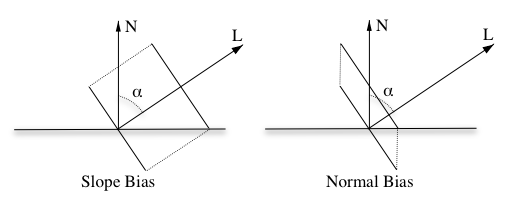
For these biases to work well it's important to scale their magnitude correctly based on the surface normal and light direction. In particular, the slope-scale bias should be proportional to the tangent of the angle between the normal (N) and the light direction (L), and the normal bias should be proportional to the sine:
float2 get_shadow_offsets(float3 N, float3 L) {
    float cos_alpha = saturate(dot(N, L));
    float offset_scale_N = sqrt(1 - cos_alpha*cos_alpha); // sin(acos(L·N))
    float offset_scale_L = offset_scale_N / cos_alpha;    // tan(acos(L·N))
    return float2(offset_scale_N, min(2, offset_scale_L));
}
Finally, one of the disadvantages of the normal bias is that it does not only bias the depth, it also offsets the shadow. On its own this offset is not very noticeable, but the offset amount is different for each of the cascades and that results in an obvious shift between cascades. Blending the cascades helps, but to reduce the problem further we also interpolate the magnitude of the bias from one cascade to the next, so that the shift is barely noticeable.
Coming Next
In part 2, I'll describe our cascade placement algorithm and finish with the optimizations that we use in order to speed up shadow map rendering.
Should that “poison” distribution be “Poisson”?
Of course. Thanks for the catch!
Thanks for the post Ignacio!
I’d been meaning to write up some thoughts on shadow cascade placement too, but you’ll probably beat me to it. In any case, I look forward to part 2. :)
Michal Valient also did a good job of collecting some tricks here:
http://www.dimension3.sk/2012/09/siggraph-2012-talk-shadows-in-games-practical-considerations/
(It’s not quite a “random” PowerPoint, given that it was in the Efficient Real-Time Shadows SIGGRAPH course.)
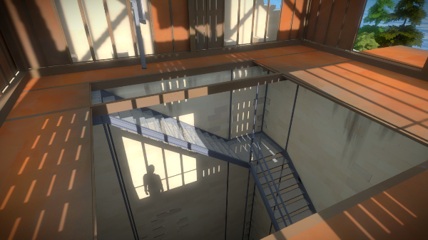
Thanks for interesting post, I will be happy to read part 2. Anyways, I see from the picture you posted that we may consider that “The Withness” is definetly human and for 90% a male :D
I also noticed that. I think most people had already assumed the character to be human, but the fact that he has a proper shadow that will probably be seen more than once in the game makes it even more realistic and immersive. Even though you don’t see the character directly, you see their outline and it enhances the idea that you really are wandering around an island.
This makes me wonder, might there be any mirrors in the game?
Well, there is definetly water :) It depends on how much it will reflect I guess.. and I would say that there are mirors( I think that light beam is bounced by some mirror(s) is some video) but the question is, if there will be mirrors tiltet to the angle you could see yourself.. maybe at the end of the game ? :D
“For the most part it is scattered in obscure power point presentations, random some blog posts,[…]”
You probably haven’t sumbled over Real-Time Shadows: http://www.amazon.de/Real-Time-Shadows-Elmar-Eisemann/dp/1568814380/ref=pd_sim_eb_5 ;)
I can really recommend this one.
Great post! Really thrilled to see that shadow, very exciting!
I was wandering if a mixed system of shadow volumes for achitechture and shadow maps for vegetation would be better given the sleek design of some interiors… But i’m a complete newbie as long as shadows are concerned.
The Witness Update on the Playstation Blog!!
http://blog.us.playstation.com/2013/10/16/the-witness-on-ps4-tiny-details-in-a-very-big-world/
Hemlock Drew, giving you the news you want!
Hm… I don’t know what the structure that is casting a shadow in this screenshot looks like. But based on what one can see, I would assume that the distance between the shadow caster and the shadow catcher on the top left is smaller than the distance in the center of the image (where the character’s silhoutte can be seen). Yet, the character’s shadow appears to be ultra-crisp versus the shape top left being blurry. But obviously, shadows should get softer with growing distance between shadow caster and catcher, not the other way around?
But… as I said in the beginning… maybe whatever casts a shadow on the top left is further away than I would assume. Or maybe this is even a WIP screenshot from when you were still figuring things out?
At any rate – love these little bits of actual development documentation that you guys release here sometimes!
I am so excited to play this game when it comes out. The Witness is one of the few games I am looking forward to in 2014.
Thanks for a very interesting and informative article. I’m very late to the party but one thing that worked for me in the past is a simple hybrid between
normal offset and slope scaled depth bias. I don’t modify vertices at all because it creates problems on its own. Rather, I simply push depth values proportionally to sqrt(1 – viewNormal.z * viewNormal.z) where viewNormal is a surface normal transformed to light’s view space. This is something that can be easily calculated in vertex shader while rendering shadow map. It still doesn’t resolve sampling artifacts at grazing angles (I believe no “traditional” method really does) but it generates usable depth biases to such degree that using other types of bias is often not even necessary. Where grazing angle artifacts are considered a problem I simply attenuate shadows at such angles in my lighting pass.